How To Make A Cover Page In Excel

Much of the data that y'all apply Excel to analyze comes in a list grade. You might need to sort the information, filter it, sum it, and perhaps fifty-fifty nautical chart it. Excel tables provide superior tools for working with data in list class.

If yous desire to sum columns of data automatically so that the totals show only the sum of visible cells (for instance), Excel's Tables features can exercise information technology. And if y'all want to format whatever Excel data in simply a couple of quick steps, Excel's Tables features can handle that task, also. And as for using a form instead of punching numbers into ordinary spreadsheet cells, Tables once over again can do the job.

Here are my top x secrets for managing lists of data using Excel Tables.

1. Create a Table in Any of Several Ways

You can create a table from the Insert tab or (as here) from the Dwelling tab, where you tin choose a style at the same fourth dimension.

The first step in learning how to work with Excel'south Tables features is to utilise the program to create a tabular array. Y'all'll demand a listing with column headings and (if you wish) row headings. Select the data, including the heading rows and columns, and click Insert > Table. Visually confirm that the range y'all've selected is correct, click the My table has headers checkbox, and click OK. Excel will then create a formatted table for you. If you would adopt to choose a item table format, select the same data area and click Home (instead of Insert); then choose a table style from the Table Styles gallery.

2. Remove the Filter Arrows

Microsoft

Click the Filter selection to toggle the display of the filter arrows on or off.

When you desire to employ some features of an Excel table, merely y'all don't plan to filter or sort your data, you lot tin can hide the filter arrows. To practise this, click somewhere within the table and and so click Data > Sort & Filter > Filter. Now yous can toggle betwixt hiding the arrows with one click and revealing them with the next. The shortcut keystroke combination Shift-Ctrl-L accomplishes the same thing.

3. Take the Format just Ditch the Tabular array

Formatting data as an Excel tabular array is the quickest style to achieve a neatly formatted range of cells in Excel. The only potential problem is that it may seem that you can't get the formatting without getting all the unwanted tabular array features likewise. Simply while this limitation is technically true, you don't have to go along the table features if you don't want them. To borrow a table style for any worksheet, first create the information as a table, making sure to cull your preferred table style for formatting it.

Adjacent, click inside the table and and then click Table Tools > Pattern > Convert to Range. Click Yes when Excel prompts yous with 'Do you desire to convert the table to a normal range?' and the table will revert to being a regular range—simply with its bonny formatting intact.

four. Gear up Ugly Cavalcade Headings

The filter arrows in an Excel table's cavalcade headings look downright ugly when those headings are right-justified. The arrows cover the rightmost characters in the headings, and there is no obvious way to fix the trouble. The workaround is to indent the content from the right side of the cell. To practise this, select the cells containing the headings that are partly subconscious and click Dwelling house > Increase Indent. If the cell contents respond past jumping to the left edge of the cell, click Dwelling > Align Right to return them to right justification. Click Increase Indent more than once as necessary to position the heading text well articulate of the filter arrows.

v. Add New Rows to a Tabular array

Rows in a table behave a trivial differently from rows in a regular worksheet. If you need to add a new row to a table, and if the Totals row is not visible, click in the bottom right cell in the table and printing the Tab key. This simple process adds a new row to the table, just as it would if you were working with a Discussion table.

To add a new row inside a table, utilize the special insert options that appear only when you've selected a prison cell inside a table.

To add rows to the end of a table, drag the small indicator in the lesser right corner of the tabular array to add more than rows and more than side by side columns, if desired. To add a row inside a tabular array, click in a prison cell either higher up or beneath where the row should be inserted and click either Home > Insert > Insert Table Row Above or Dwelling house > Insert > Insert Table Row Below, depending on where you want the new row to appear. The table'southward formatting volition automatically accommodate and so that the new row is correctly formatted.

Next page: How to calculate accurate column totals.

6. Calculate Accurate Totals

When you choose to total a cavalcade in a tabular array, Excel will add a SUBTOTAL function that totals only the values in visible cells.

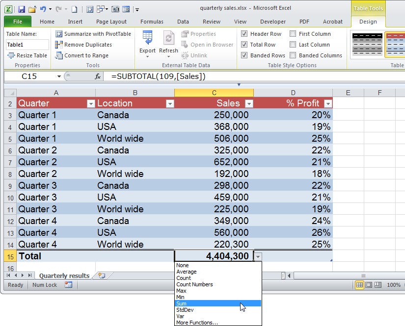
Anyone who has ever tried to utilise the SUM function to total a cavalcade of data in which some of the rows are subconscious has received a nasty surprise: The SUM office calculates the total of all of the cells in a range, whether they're visible or not. This characteristic of the office means that the consequence won't be the total of the numbers in the visible rows—and that discrepancy tin can be a huge problem. The way tyo avoid this difficulty is to use the SUBTOTAL part instead. Excel volition do this automatically when y'all apply its Full row feature for your table.

When you desire to add together a total row to the tabular array, click inside the table, right-click, and choose Table > Totals Row; or click within the table and click Table Tools > Design > Full Row. In either example, a full row volition appear at the foot of the table. If the last column contains numerical values, Excel volition automatically employ a SUBTOTAL function to sum them.

To add together a total to any other column, click in the advisable cell in the Total row, and in the drop-downward menu click SUM. This performance will add a SUBTOTAL formula to the prison cell that volition total only visible values when the tabular array is filtered. Yous may choose other calculation options from this drop-downward listing, including Min, Max, Count, and Average.

7. Create a Chart From Table Data

Charts created from Excel tables automatically expand and contract as you add information to or remove data from the table.

Ane significant benefit of formatting a list equally a table is that charts created from table data change dynamically when you add data to or remove data from the tabular array. Then a column chart that charts the values in a range will expand to comprise new values when you add together them to the table. This is the instance whether you add data to the lesser of the table or innovate a new column to the correct of it. Creating a nautical chart based on the table is the aforementioned as creating any chart in Excel—only the beliefs of the chart is different. Tables of this type are extremely useful when y'all work with information that expands or contracts over time.

8. Enter Data Using a Simple Form

Excel'south subconscious Form feature creates a data entry grade for your table automatically.

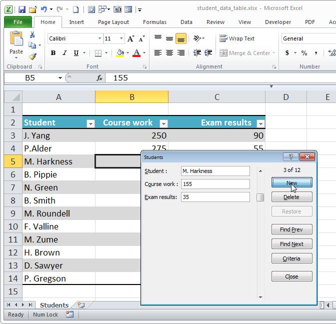
Typing lots of data across a wide table can exist quite cumbersome; oftentimes, entering data into a form is easier. Earlier versions of Excel included a handy Grade tool; that tool is still available, merely you won't notice it on the Ribbon. To make it easier to find, you can add information technology to Excel'southward Quick Access Toolbar: Click File > Options > Quick Admission Toolbar. In the Choose Commands From listing, click All Commands then scroll downwardly and click Form…. Click Add to add together the tool to the Quick Admission Toolbar, and then click OK.

To use the form, click somewhere within your table and then click the Form push to display a form dialog area. The form heading is the sheet name, and the grade contains boxes where you lot can preview the current course information and add new data. To add new data, click New and blazon the data into the relevant text boxes. To view the course data, click Find Prev or Find Next to move through the data i row (record) at a fourth dimension. To exit the form, click Close.

ix. Sort and Filter Table Data

One primal feature of Excel's tables is their ability to sort and filter the information in the table. To perform either of these deportment, click the down arrow to the correct of any table column and then cull a Sort or Filter option. The ii Sort options bachelor are 'ascending' and 'descending'. The Filter options vary depending on whether you lot're working with a column of numbers, text, or dates.

Excel's born AutoFilters feature gives you a select range of prebuilt filters for filtering tabular array data.

You tin then select from among a number of predefined options, or click Custom Filter and build your own. Alternatively you can create complex filters such every bit AND and OR filters. For example, locating values in a column that are less than $200,000 or more $400,000 involves using an OR filter. To create it, click Custom Filter and and then build both parts of the search in the dialog area, making certain to click the OR pick. Similarly you can create AND filters that work across two columns, thereby enabling you to display information such as "All entries for Canada, where sales are greater than $300,000." In this case yous would select to view only 'Canada' in the Location column. In the Sales column, click Numbers Filters > Custom Filter > is greater than, type 300000 and click OK.

Whatsoever cavalcade that has a filter in place will testify a filter icon instead of the downward-pointing triangle, and then you lot tin see at a glance where the filters are. To clear a filter, click the Filter icon and click Clear filter from; or click Abode > Sort & Filter > Clear to clear all filters from all columns in the tabular array.

10. Create Complex OR Searches Across Multiple Columns

OR searches beyond multiple columns are relatively complex and can't be generated past using the AutoFilter options.

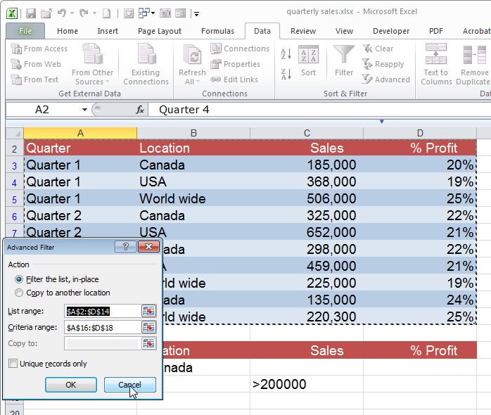
Ane type of search that y'all can't build using the menu options is an OR search of the blazon "All entries for Canada or where sales are greater than $200,000." Consequently you must write a search pedagogy of this type in a different fashion. To do and so, starting time copy the table heading row and paste information technology a few rows immediately below your tabular array. Below these headings, in the Location column, type ="=Canada" and in the 2nd row, in the Sales cavalcade, blazon >200000. Click within the table, click Data > Advanced > Filter the list, in-place. Confirm that the List range is the tabular array range, and set the Criteria Range to an area covering the second set of headings and the 2 information rows beneath information technology. And then click OK to filter the listing.

If you've enjoyed this article, check out these related stories:

• "How to Create Advanced Microsoft Excel Spreadsheets"

• "Work Faster in Microsoft Excel: ten Secret Tricks"

• "Make Data Entry Easier in Microsoft Excel: ten Tricks"

Source: https://www.pcworld.com/article/460058/10-secrets-for-creating-awesome-excel-tables.html

Posted by: rodrigueztwild1973.blogspot.com

Share this post